Applying Physics-Informed Neural Networks (PINNs): Hands-On Modeling of 2D Plates

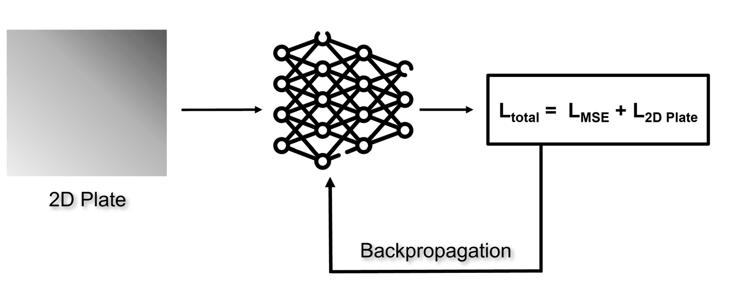
The MSE loss is the supervised loss, and 2D Plate loss is the unsupervised loss derived from the heat equation for the 2D plate

In our previous blog post, we introduced the concept of Physics Informed Neural Networks, touching upon their applications and various use-cases. Today, we'll delve further into this fascinating topic by exploring our first use-case in detail: Heat Transfer in a 2D plate.

Let's dive in...

Heat Transfer in 2D plate

For analysis purpose, let's consider a 2D metallic plate subject to boundary conditions where one edge is maintained at 1°C and the remaining edges at 0°C. While it's possible to measure the temperature at various internal points, doing so necessitates the use of a thermometer for each measurement location. This raises a critical question: how many points should we measure to accurately assess the temperature distribution? The number of thermometers needed directly correlates to the number of points selected for measurement. The challenge then is to devise a method that allows for the generalized measurement of temperature at any given point (x, y) on the plate.

A potential approach to this problem involves leveraging techniques such as Finite Element Analysis (FEA) or Finite Difference Methods (FDM). However, it's important to note that these methods are accompanied by significant computational demands and can become exceedingly complex when dealing with irregular geometries. So, what's the alternative in such scenarios?

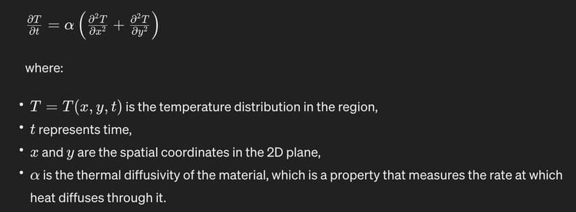
Heat Equation for 2D Plate

PINNs

Given the complexities associated with the aforementioned methodologies, Physics Informed Neural Networks (PINNs) emerge as a viable alternative. Unlike traditional methods, PINNs do not necessitate meshing the domain but instead learn the solution directly. This attribute renders them exceptionally adaptable to complex geometries without notably escalating computational complexity.

Code

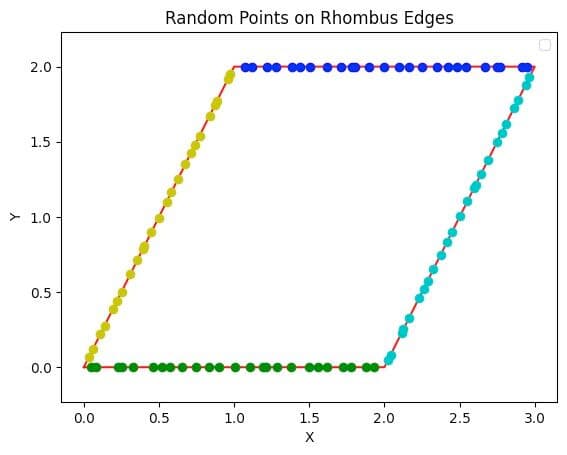
Now, let's dive into the coding segment. We'll begin by initializing boundary points with labels and selecting internal points for a rhombus. Following this, we'll construct a neural network using a fully connected architecture, which will be trained on the points we've generated. For the internal points, where labels are absent, we will calculate the loss by applying the Heat Equation specific to 2D plates. This calculated loss will then be integrated with the standard mean squared error loss function. Incorporating the Heat Equation in this manner allows the model to generate more reliable predictions for scenarios not explicitly represented in the training data, ensuring that its outputs adhere to the principles of thermodynamics.

Steps

First,we'll import the required libraries. Our model creation will leverage PyTorch, while the Latin Hypercube sampling method will be used to generate both boundary and internal points.

import numpy as np
import matplotlib.pyplot as plt
from scipy.stats.qmc import LatinHypercube

import torch
import torch.nn as nn
from torchsummary import summary
from torch.utils.data import Dataset, DataLoader

Next, we will initialize the rhombus by specifying the coordinates of its vertices. Following this, we will employ the Latin Hypercube sampling strategy to randomly select 25 points from each edge.

vertex1 = np.array([0, 0])
vertex2 = np.array([1, 2])
vertex3 = np.array([3, 2])
vertex4 = np.array([2, 0])

left_edge = np.array([vertex1, vertex2])
top_edge = np.array([vertex2, vertex3])
right_edge = np.array([vertex3, vertex4])
bottom_edge = np.array([vertex4, vertex1])

lhc = LatinHypercube(d=1)

n_samples = 25
samples = lhc.random(n=n_samples)

def get_boundary_points(edge, t_values): return [edge[0] + t * (edge[1] - edge[0]) for t in t_values]

top_points, bottom_points, left_points, right_points = [],[], [], []

top_points.extend( get_boundary_points(top_edge, samples.flatten()))
bottom_points.extend( get_boundary_points( bottom_edge, samples.flatten()))
left_points.extend( get_boundary_points(left_edge, samples.flatten()))
right_points.extend( get_boundary_points(right_edge, samples.flatten()))

Let’s now visualize the generated boundary data points.

import matplotlib.pyplot as plt

vertices = np.array([vertex1, vertex2, vertex3, vertex4, vertex1])
plt.plot(vertices[:,0], vertices[:,1], 'r-')

for point in top_points:
plt.plot(point[0], point[1], 'bo')

for point in bottom_points:
plt.plot(point[0],point[1], 'go')

for point in left_points:
plt.plot(point[0], point[1], 'yo')

for point in right_points:
plt.plot(point[0], point[1], 'co')

plt.xlabel('X')
plt.ylabel('Y')
plt.title('Random Points on Rhombus Edges')
plt.axis('equal')
plt.legend()
plt.show()

To generate the internal points, we will apply a geometric approach. Initially, the rhombus will be divided into two triangles. Subsequently, we will randomly generate 10,000 points within one of these triangles, which will then serve as the internal points of the rhombus.

def random_point_in_triangle(v1, v2, v3):
weights = np.random.rand(3)
weights /= weights.sum()
x = weights[0] * v1[0] + weights[1] * v2[0] + weights[2] * v3[0]
y = weights[0] * v1[1] + weights[1] * v2[1] + weights[2] * v3[1]
return [x, y]

def generate_random_points_in_ rhombus ( vertex1, vertex2, vertex3, vertex4, n):
points = []
for _ in range(n):
if np.random.rand() < 0.5:
point = random_point_in_triangle(vertex1, vertex2, vertex3)
else:
point = random_point_in_triangle(vertex1, vertex3, vertex4)
points.append(point)
return np.array(points)

internal_points = generate_random_points_in_ rhombus (vertex1, vertex2, vertex3, vertex4, 10000)

Next, we will create a Dataset class based on PyTorch.

class EdgePointsDataset(Dataset):
def __init__(self, points):
self.X = torch.tensor( points[0].astype(np.float32 ))
self.y = torch.tensor( points[1].astype(np.float32 ))

def __len__(self):
return len(self.X)

def __getitem__(self, idx):
return self.X[idx], self.y[idx]

class InternalPointsDataset(Dataset):
def __init__(self, X):
self.X = torch.tensor(X.astype(np.float32), requires_grad=True)

def __len__(self):
return len(self.X)

def __getitem__(self, idx):
return self.X[idx]

Then, we will create a DataLoader for the Dataset classes we established in the previous step.

# Creating points list
edge_points_X = np.array(top_points + bottom_points + left_points + right_points) edge_points_y = np.array([[1.0]]*len(top_points) + [[0.0]]*len(bottom_points) + [[0.0]]*len(left_points) + [[0.0]]*len(right_points)) edge_points = [edge_points_X, edge_points_y]

# Dataset class
edge_points_dataset = EdgePointsDataset(edge_points)
internal_points_dataset = InternalPointsDataset( internal_points)

# Dataloader
edge_points_dataloader = DataLoader(edge_points_dataset, batch_size=10, shuffle=True)
internal_points_dataloader = DataLoader( internal_points_dataset, batch_size=1000, shuffle=True)

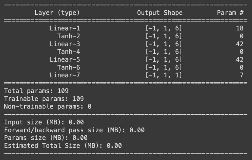
Now, we will define the model class, which will include two hidden layers, one input layer, and one output layer.

class NeuralNet(nn.Module):
def __init__(self, input_neurons, hidden_neurons, output_neurons):
super(NeuralNet, self).__init__()
self.input_shape = input_neurons
self.output_shape = output_neurons
self.hidden_neurons = hidden_neurons

self.input_layer = nn.Linear(input_neurons, hidden_neurons)
self.hidden_layer1 = nn.Linear(hidden_neurons, hidden_neurons)
self.hidden_layer2 = nn.Linear(hidden_neurons, hidden_neurons)
self.output_layer = nn.Linear(hidden_neurons, output_neurons)

self.tanh = nn.Tanh()

def forward(self, x):
x = self.input_layer(x)
x = self.tanh(x)
x = self.hidden_layer1(x)
x = self.tanh(x)
x = self.hidden_layer2(x)
x = self.tanh(x)
x = self.output_layer(x)

return x

Next, we will introduce an optimizer and define the loss function, preparing us to commence the model's training. The following summary provides an overview of the model architecture, including the count of trainable parameters.

device = 'cuda' if torch.cuda.is_available() else 'cpu'
model = NeuralNet(2,6,1).to(device)
optimizer = torch.optim.Adam( model.parameters(), lr = 5e-4)
loss_fn = nn.MSELoss()
summary(model, (1, 2))

The final step involves training the model. Within the training loop, you'll notice that we incorporate the heat equation by utilizing the torch.autograd.grad() function. This function calculates the derivative of the output with respect to the input points, and this derivative is then integrated into the loss function.

loss_values = []
epoch = 10000

for i in range(epoch):
total_loss, edge_loss_total, internal_points_loss_total = 0.0, 0.0, 0.0
for (edge_points, temp), internal_points in zip(edge_points_dataloader, internal_points_dataloader):
optimizer.zero_grad()

edge_points = edge_points.to(device)
temp = temp.to(device)
out = model(edge_points)
edge_points_loss = loss_fn(out, temp)

internal_points = internal_points.to(device)
out_internal = model(internal_points)
du_dx = torch.autograd.grad(out_internal, internal_points, torch.ones_like(out_internal), create_graph=True)[0][:, 0]
du2_dx2 = torch.autograd.grad(du_dx, internal_points, torch.ones_like(du_dx), create_graph=True)[0][:, 0]
du_dy = torch.autograd.grad(out_internal, internal_points, torch.ones_like(out_internal), create_graph=True)[0][:, 1]
du2_dy2 = torch.autograd.grad(du_dy, internal_points, torch.ones_like(du_dy), create_graph=True)[0][:, 1]

physics = du2_dx2 + du2_dy2
internal_points_loss = torch.mean(physics**2)

loss = edge_points_loss + internal_points_loss

loss.backward()
optimizer.step()
total_loss += loss.item()
edge_loss_total += edge_points_loss.item()
internal_points_loss_total += internal_points_loss.item()

loss_values.append(total_loss)
if (i+1) % 1000 == 0:

plt.semilogy(loss_values)
plt.legend()

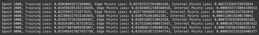
As we do multiple epochs, the loss reduces and the nearwork learns how heat is propagated on a 2D plate.

The decreasing loss values indicate that the model is successfully learning the pattern of heat transfer.

In this post, we explored the principles of heat transfer in a 2D plate and detailed the process of coding and training a neural network in Python to model these principles.

I hope you found it insightful and enjoyable.

In the next post, we will discuss the more complex case of heat transfer in the case of a lid-driven cavity.